Multidimensional scaling for Clusterpath.

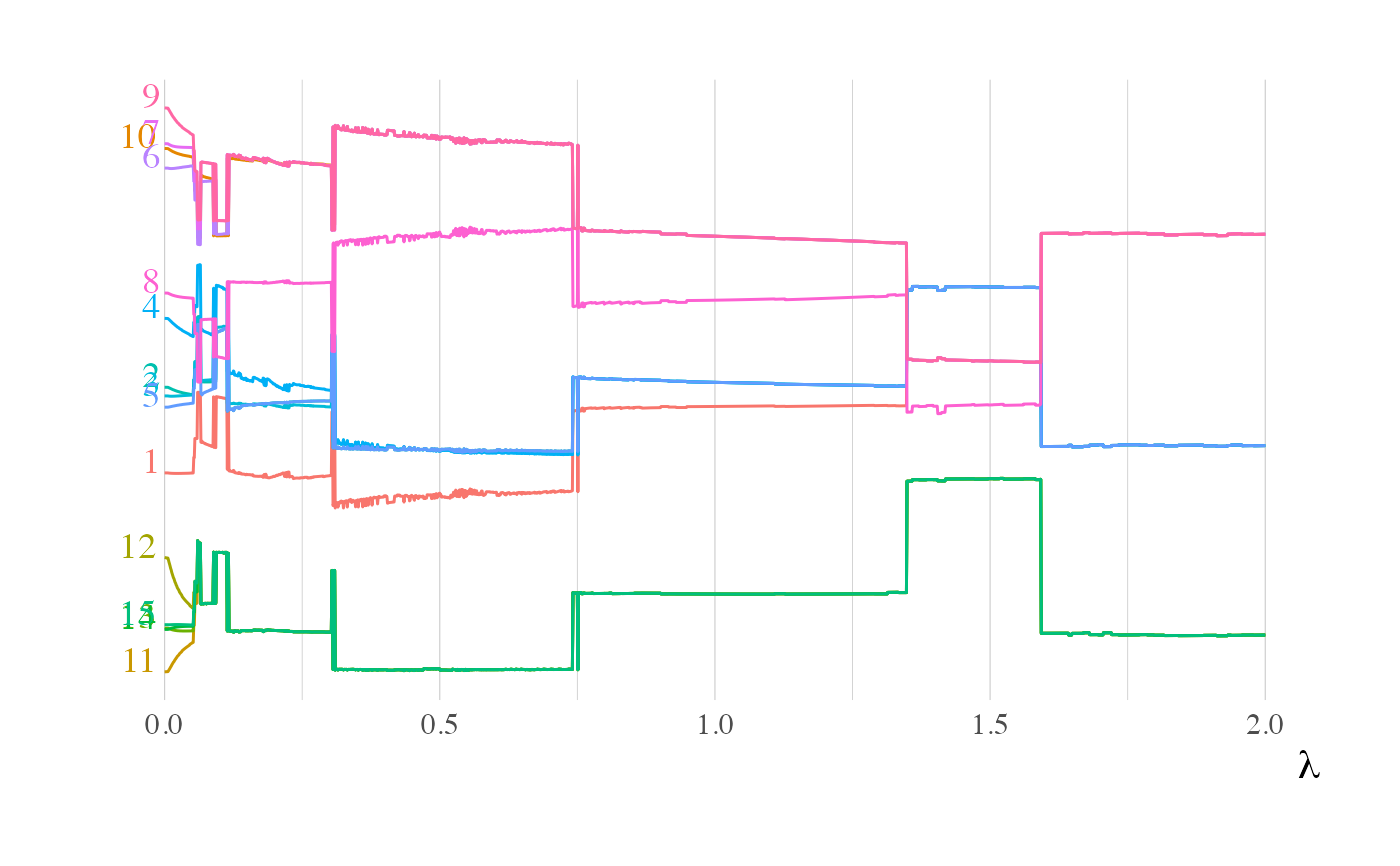
Visual representation of the distance evolution between the clusters along \(\lambda\). We recall that for a precision matrix \(\Theta\) which have a block matrix structure, the distance between two variables is defined by: $$ D(\Theta_{i\cdot}, \Theta_{j\cdot}) = \sqrt{\sum_{k\neq i,j} (\Theta_{ik} - \Theta_{jk})^2}, $$ With this distance, two variables in the same cluster have a null distance.

Usage

ggdistance(list_results, names = NULL)

Arguments

list_results

A list of results optimization from HR_Clusterpath().

names

A list of name : the names of the variables, if NULL it will be \(1,...,d\).

Method used for the representation

The cluster's distance is a measure of dissimilarities between variable. With this in mind, we have a dissimilarities matrix \(W\) and we want to build for each \(\lambda\) a reconstition of a 1-dimensional scatter plot with the respect of these dissimilarities.

We use the function cmdscale() from stats package to operate the optimization. It follows the analysis of \([1]\).

References

\([1]\) Some properties of clasical multi-dimesional scaling K.V. Mardia

Examples

# Construction of clusters and R matrix
R <- matrix(c(1, -3, 0,
              -3, 2, -2,
              0, -2, 1), nc = 3)
clusters <- list(1:5, 6:10, 11:15)

# Construction of induced theta and corresponding variogram gamma
Theta <- build_theta(R, clusters)
Gamma <- graphicalExtremes::Theta2Gamma(Theta)

gr3_bal_sim_param_cluster <-
  list(
    R = R,
    clusters = clusters,
    Theta = Theta,
    Gamma = Gamma,
    chi = 1,
    n = 1e3,
    d = 15
  )

set.seed(804)
data <- graphicalExtremes::rmpareto(n = gr3_bal_sim_param_cluster$n,
                                    model = "HR",
                                    par = gr3_bal_sim_param_cluster$Gamma)

lambda <- seq(0, 2, 1e-3)

res <- HR_Clusterpath(data = data,
                      zeta = gr3_bal_sim_param_cluster$chi,
                      lambda = lambda,
                      eps_f = 1e-1)

ggdistance(res)